
Excel has many uses and one of them is to create a list that can be displayed and then selected. Creating adrop-down list in Excelwill help users or workers to be more efficient when using this spreadsheet.
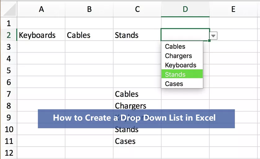
How to Create a Drop Down List in Excel
These work in a simple way, as it allows a user to choose an item from the list automatically. Here’s a step-by-step guide to create a Drop Down list in excel.
Steps to make a drop-down list in Excel:
Step 1: Once the entry is created in a new spreadsheet, click and drag where you want the drop-down list to appear. In this case there is a column of animals and the other column will be their type of food, in the latter I will display the list, therefore I select it.
Step 2:Once selected (and make sure it is selected where you want the list) go to the tab at the top where it says “Data” then “Data validation” the latter is a small button found in ” data tools ”Here you can see its icon and location:
Step 3:Once you enter “data validation” this box will appear. Go to the upper tab that says “configuration” there choose the option from the table “Allow” that says “list”
And at the bottom, where it says “Origin” select the list of data that goes in the second column. The list that you want to appear in the second column (In this case in “Types of animals”) must be written to one side, in a column of the same spreadsheet. Click on the button that appears next to “Origin”:
Once there, a thin box will appear, and the list of data to be displayed must be selected. In this case, that list is “Herbivores, Carnivores and Omnivores”.
You can write as much data as you wish to appear in theExcel drop-down list. Once selected, click on the right button of “data validation” and then on the main big box on “Accept”
Step 4:An arrow must have been placed in the upper right part of the box, which when clicking on it opens a selective menu, said arrow should look like this:
By clicking on that arrow, you can see that the data previously placed on the right side, which has previously been selected (“Herbivores, Carnivores and Omnivores”), is displayed.
Step 5:As a last step, you only have to select all the elements that are shown in the drop-down list. You can place all the elements you want.
The important thing is to follow the steps correctly to avoid mistakes or confusion. In this simple way it has been possible to create adrop-down list in Excel.